5.2 Hydraulics of Flow in Unconfined Aquifers
Groundwater flow in unconfined aquifers obeys the same principles as flow in confined aquifers with an added element: the elevation of the top of the saturated zone defines a water table, which is the elevation of water that stands in a screened well just deep enough to encounter water. An equipotential contour connects points of equal hydraulic head. The water table itself is not an equipotential line; it has a variable head because it varies in elevation.
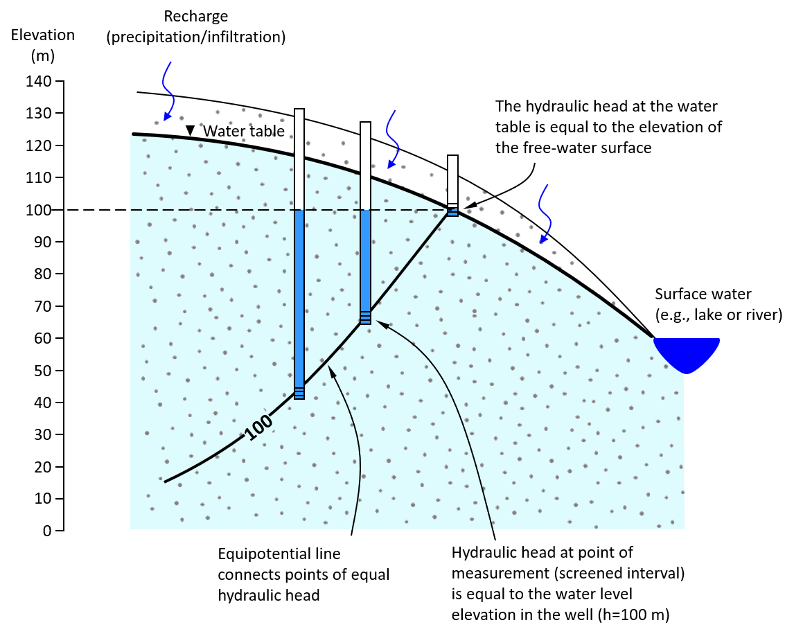 Figure 21 – Equipotential contours in an unconfined aquifer; the contour lines connect points of equal hydraulic head and extend to the water table of the same elevation (Cohen and Cherry, 2020).
At the field scale, hydraulic head can be measured using wells. The cross-section for this problem shows an upper unconfined aquifer, a clay aquitard, and a lower confined aquifer. Surface water bodies at both ends act as constant-head boundaries. In practice, horizontal flow in unconfined aquifers is often approximated as purely horizontal, and the water table can be approximated as a planar surface when assessed away from boundary conditions (see Figure 25).
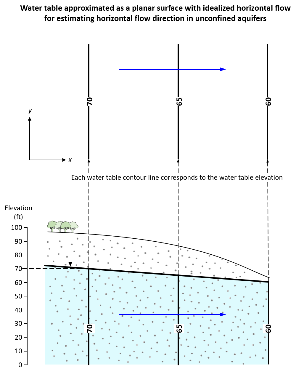 Figure 25 – Water table represented as a planar surface with predominantly horizontal flow throughout the cross section (Cohen and Cherry, 2020).
Example Problem 9
Estimate the water level in each well and determine if there is vertical flow through the clay aquitard. Consider a system where a horizontal confined aquifer beneath a clay layer is bounded on both sides by constant head boundaries, which correspond to the water level elevations in the unconfined water bodies at the left and right.
Interactive exercise
Exercise 9: Horizontal Flow and Multiple Aquifers
Estimate water levels, determine vertical flow, and experiment with constant head boundaries.
Step 1: Estimate Levels and Determine Vertical Flow
Consider an unconfined aquifer over a clay aquitard, and a confined aquifer below. The system is flanked by water bodies (54 m on the left, 50 m on the right). Assuming a linear decrease in the water table, estimate the level in each well (Left, Center, Right) and determine whether there is vertical flow through the clay.
Conceptual Hint
If the water table decreases linearly from 54 m to 50 m, what are the heads at 1/4, 1/2, and 3/4 of the distance? Now compare those values with the heads in the lower confined aquifer — both share the same constant head boundaries. If the head is equal above and below the clay at each location, is there a vertical gradient?
Visual Simulation
Show solution
Problem 9 Solution
Step 1: As an approximation, assume the water table is linear. By linear interpolation, the water level in the center is 52 m. The well on the right is half the distance from the right side to the middle, so the water level is 51 m. Similarly, the water table elevation at the location of the well on the left side is 53 m.
Step 2: The horizontal confined aquifer beneath the clay is bounded on both sides by constant head boundaries, the values of which correspond to the water level elevation in each water body (see analogous scenarios). Flow is horizontal based on the geometry of the confined aquifer and the position of the boundaries (on either end).
Step 3: The medium is homogeneous, so the gradient is constant, meaning that the spacing between the equipotential lines is constant. The spacing between the lines and their values are determined by linear interpolation.
Step 4: The well on the left side is screened in the confined aquifer where the head is 53 m. At this same location, the water table elevation is also 53 m. We simplified by assuming a linear decline of the water table. Because we are assuming a linear gradient in both the confined and unconfined aquifer, the head at each location will be the same above and below the clay. As a result, there is no vertical gradient and so, no vertical flow across the clay.
Conceptual Connections
- Compare this exercise with Exercise 7, which also analyzes vertical flow through a low-K layer — but in a lake-sediment-aquifer system. The key difference: in Exercise 7, the confined aquifer and the lake have different boundary heads, creating a vertical gradient. In Exercise 9, both aquifers share the same boundary heads, so the vertical gradient is zero.
- Compare with Exercise 12, where upward flow occurs through a clay aquitard. In Exercise 12, the potentiometric head in the lower confined aquifer (40 m) exceeds the water table in the upper unconfined aquifer (~38 m), creating an upward vertical gradient. Exercise 9 represents the special case where heads are perfectly balanced.
- The condition of zero vertical flow across an aquitard requires that the hydraulic head above equals the hydraulic head below at every horizontal position. This is an idealized scenario; in real aquifers, slight differences in boundary conditions, heterogeneity, or recharge/discharge create small but non-zero vertical gradients.
- This exercise illustrates why nested or multi-port wells are essential for hydrogeological characterization: without measuring head at multiple depths, one might incorrectly assume vertical flow exists based on water table measurements alone.