Groundwater flow in unconfined aquifers obeys the same principles as flow in confined aquifers with an added element: the elevation of the top of the saturated zone defines a water table, which is the elevation of water that stands in a screened well just deep enough to encounter standing water. For example, the hydraulic head of the water table intersected by a shallow well is the water level measured in that well.
An equipotential contour connects points of equal hydraulic head, which is measured using wells (field-scale piezometers). The water table itself is not an equipotential line; it has a variable head because it varies in elevation.
Importantly, a body of surface water such as a lake acts as a constant-head boundary. The water level in the lake is the same everywhere, so the entire lake shoreline represents a single equipotential line. Because groundwater flow is perpendicular to equipotential lines (in isotropic media), flow lines must approach the lake shore at roughly right angles.
 Figure 22 – Potentiometric cross section, groundwater flow direction, and water table contour map in an idealized unconfined aquifer. The contour map represents the topography of the water table and can be used to infer the general direction of flow (Cohen and Cherry, 2020).
Example Problem 8
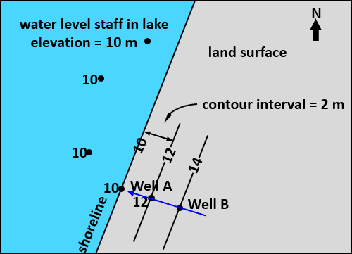
The figure below is a map view of a lake and shoreline. The water table elevation at Well A is 12 m. Assuming the water table is planar (an inclined plane), what is the expected water level elevation in Well B?
Interactive exercise
Simulation: Water Table and Equipotential Lines
Step 1: Determine the Water Level
The figure shows a map view of a lake and its shoreline. The water table elevation at Well A is 12 m. Assuming the water table is planar (an inclined plane) and the lake elevation is 10 m, what is the expected water level elevation in Well B?
Observe the map: the lake is at 10 m and Well A at 12 m. Buttons will activate in a few seconds...
Show solution
Problem 8 Solution
The correct answer is 14 m.
The water level in the lake is horizontal at 10 m. Therefore, the hydraulic head is the same everywhere in the lake, including along the entire lake–shoreline interface. This shoreline is a 10 m equipotential line.
Well A is located at a certain perpendicular distance from the shoreline and has a head of 12 m. This means the contour interval between the shoreline (10 m) and Well A is 2 m. Because the water table is assumed planar, the gradient is constant: every time you move the same perpendicular distance away from the shore, the head increases by another 2 m.
Well B is located at roughly twice the perpendicular distance from the shoreline compared with Well A. Therefore, the head at Well B must be 10 m + (2 × 2 m) = 14 m.
Why the other choices are wrong:
12 m — This would only be true if Well B were at the same distance from the shoreline as Well A, which it is not.
13 m — This assumes the head increases by 1 m over the distance from A to B, ignoring that the lake itself is the 10 m reference and the interval from shore to A is already 2 m.
A value between 12 and 13 m — This underestimates the planar gradient; the doubling of distance from the constant-head boundary produces a doubling of head difference.